Poi Pad: OpenOffice Basic Formula Tutorial

How to use different formula in Open Office

OpenOffice.org or OpenOffice is an open-source office suite and was the latter version of StarOffice. Just like the Microsoft Office, it contained word processor (Writer), a spreadsheet (Calc), a presentation application (Impress), a drawing application (Draw), a formula editor (Math), and a database management application (Base) and a wide variety of file format that can be read by the OpenOffice.

OpenOfice Calculator (Calc) Spreadsheet provides useful functions to have a quick and easy way calculation. This tutorial includes step by step examples of how to use common functions featured in Open Office Calc.

In computing grades, OpenOffice Calc is useful. Average function is used to find the average value for a range of number.

To get the AVERAGE, simply type equal sign (=) AVERAGE, then drag the cells you want to find the average and enclosed it with parenthesis and click ENTER.

* dragging down through the column makes it easier.

VLOOKUP (Vertical LookUp) is used to find specific information that has been stored in a spreadsheet table. VLOOKUP can help you find data that matches specific criteria.

To indicate the grade based on the average, create a range and its corresponding grade (legend).

Simply click the FUNCTION Key (fx) and search the VLOOKUP or manually type it in the Formula bar. The VLOOKUP function checks if a specific value is contained in the first column of an array. The function then returns the value in the same row of the column named by Index.

Using the VLOOKUP formula in OpenOffice, the final grade can be computed by typing the =VLOOKUP, then drag the column “average" (table lookup) . Select the range and legend columns as your table array putting the Dollar symbol ($) makes it absolute. Column index number is in row number two, and range look up is your logical value if its TRUE or FALSE.

lookup value.This argument is the value that is searched for in the first column of the table array. The lookup value can be a text string, a logical value (TRUE or FALSE only), a number, or a cell reference to a value.

table array. This is the range of data that the function searches to find your information. The table_array must contain at least two columns of data. The first column contains the lookup values. These values can be text, numbers, or logical values. This argument is a named range or a reference to a range of cells.

To get the total number of students depending on their grade range, simply type =COUNTIF, then drag the column of FINAL grade then indicate comma and click the column of the corresponding grade.

To get the percentage between grade range type = then click the COUNT column and divide (/) it to the total number of students , enclosed with parenthesis.

If you wish to change the passing grade, an efficient way to do that is to increment the value of your data.

Changing the set passing grade is made easier by computing the increment based on the set passing grade. Simply type = sign, 100(perfect score) less than the passing grade and then divide it to the number of your range (10).

Given here in the figure, the passing grade is 80. To increment the values of your data, click the cell of the passing grade then add the increment value by clicking the cells of your computed increment value.

The succeeding value for the other range is incremented by clicking the above value and then adding the computed increment value.

Here the passing grade is 60, values were incremented from a grade of 2.25 to 2.

In this figure, the set passing grade is 80, so the grade were from 2.25 to 5.

Increment in the value of your data is much easier to do, because this will automatically change your whole data based on your set passing grade.

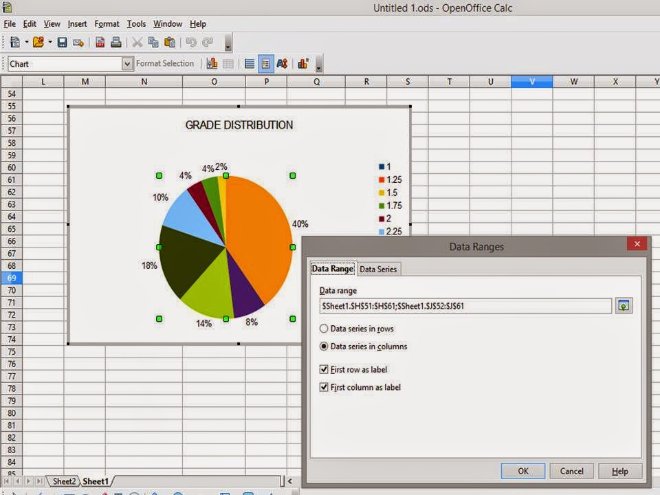
To create graph or chart that will represent your data, just click the chart icon, a chart wizard will pop where you can choose a variety of chart types to use.